2. PRINCIPLES
2.1. Model components
|
The study area is divided into a nodal network of triangles, rectangles, or any other polygons with a maximum of 6 sides. The model consists further of three parts: -a. An agronomic water balance model, which calculates for each polygon the downward and upward water fluxes in the soil profile depending on the fluctuations of the water table; -b. A ground water model of the aquifer, which calculates the groundwater flows into and from each polygon and the ground water levels per polygon depending on the upward and downward water fluxes. The parts 1 and 2 are interactive as they influence each other. -c. A salt balance model which runs parallel to the water balance model and determines the salt concentrations in the soil profile, and of the drainage, well and groundwater. These parts are discussed in sect. 3, 4 and 5 respectively. Some features of generalimportance are mentioned below. 2.2. Polygonal network The model permits a maximum of 240 internal and 120 external polygons with a minimum of 3 and a maximum of 6 sides each. The subdivision of the area into polygons, based on nodal points with known co-ordinates, should be governed by the characteristics of the distributionof the cropping, irrigation, drainage and ground water characteristics over the study area. The nodes must be numbered, which can be done at will. With an index one indicates whetherthe node is internal or external. Nodes can be added and removed at will or changed frominternal to external or vice versa. Through another index one indicates whether the internalnodes have an unconfined or semi-confined aquifer. This can also be changed at will. Nodal network relations are to be given indicating the neighbouring polygon numbers of each node. The program then calculates the surface area of each polygon, the distancebetween the nodes and the length of the sides between them using the Thiessen principle.Hydraulic conductivity can vary for each side of the polygons. The depth of the water table, the rainfall and salt concentrations of the deeper layersare assumed to be the same over the whole polygon. Other parameters can very within thepolygons according to type of crops and cropping rotation schedule (sect. 2.5). |
|
2.3. Seasonal approach
The model is based on seasonal input data and returns seasonal outputs. The number of seasons per year can be chosen between a minimum of one and a maximum of four. One can distinguish for example dry, wet, cold, hot, irrigation or fallow seasons. Reasons of not using smaller input/output periods are:
-a. short-term (e.g. daily) inputs would require much information, which, in large areas may not be readily available;
-b. short-term outputs would lead to immense output files, which would be difficult to manage and interpret;
-c. this model is especially developed to predict long term trends, and predictions for the future are more reliably made on a seasonal (long term) than on a daily (short term)
basis, due to the high variability of short term data;
-d. though the precision of the predictions for the future may be limited, a lot is gained when the trend is sufficiently clear. For example, it need not be a major constraint to
the design of appropriate salinity control measures when a certain salinity level, predicted by Sahysmod to occur after 20 years, will in reality occur after 15 or 25 years.
2.4. Computational time steps
Many water balance factors depend on the level of the water table, which again depends onsome of the water balance factors. Due to these mutual influences there can be non-linearchanges throughout the season. Therefore, the computer program performs daily calculations.For this purpose, the seasonal water-balance factors given with the input are reducedautomatically to daily values. The calculated seasonal water-balance factors, as given inthe output, are obtained by summations of the daily calculated values. Ground-water levelsand soil salinity (the state variables) at the end of the season are found by accumulatingthe daily changes of water and salt storage.
In some cases the program may detect that the time step must be taken less than 1 day forbetter accuracy. The necessary adjustments are made automatically.
2.5. Hydrological data
|
The method uses seasonal water balance components as input data. These are related to thesurface hydrology (like rainfall, potential evaporation, irrigation, use of drain and wellwater for irrigation, runoff), and the aquifer hydrology (e.g. pumping from wells). Theother water balance components (like actual evaporation, downward percolation, upward capillary rise, subsurface drainage, ground water flows) are given as output. The quantity of drainage water, as output, is determined by two drainage intensity factors for drainage above and below drain level respectively (to be given with the input data) and the height of the water table above the given drain level. This height results from the computed water balance Further, a drainage reduction factor can be applied to simulate a limited operation of the drainage system. Variation of the drainage intensity factors and the drainage reduction factor gives the opportunity to simulate the impact of different drainageoptions. To obtain accuracy in the computations of the groundwater flow (sect. 2.8), the actualevaporation and the capillary rise, the computer calculations are done on a daily basis.For this purpose, the seasonal hydrological data are divided by the number of days per season to obtain daily values. After the seasonal computations, the hydrological components are totalled. 2.6. Cropping patterns/rotations The input data on irrigation, evaporation, and surface runoff are to be specified per season for three kinds of agricultural practices, which can be chosen at the discretionof the user: -A: irrigated land with crops of group A -B: irrigated land with crops of group B -U: non-irrigated land with rain-fed crops or fallow land The groups, expressed in fractions of the total area, may consist of combinations of crops or just of a single kind of crop. For example, as the A-type crops one may specify the lightly irrigated cultures, and as the B type the more heavily irrigated ones, such as sugar cane and rice. But one can also take A as rice and B as sugar cane, or perhaps trees and orchards. A, B and/or U crops can be taken differently in different seasons, e.g. A=wheat plus barley in winter and A=maize in summer while B=vegetables in winter and B=cotton in summer. Non-irrigated land can be specified in three ways: (1) as U=1-A-B and (2) as A and/or B with zero irrigation. (3) a combination of (1) and (2) |
|
When a fraction A1, B1 and/or U1 differs from the fraction A2, B2 and/or U2 in another season, because the irrigation regime changes in the different seasons, the program will detect that a certain rotation occurs. If one wishes to avoid this, one may specify the same fractions in all seasons (A2=A1, B2=B1, U2=U1) but the crops and irrigation quantities may be different and may need to be proportionally adjusted. One may even specify irrigated land (A or B) with zero irrigation, which is the same as un-irrigated land (U).
Cropping rotation schedules vary widely in different parts of the world. Creative combinations of area fractions, rotation indices, irrigation quantities and annual input changes can accommodate many types of agricultural practices.
Variation of the area fractions and/or the rotational schedule gives the opportunity to simulate the impact of different agricultural practices on the water and salt balance.
2.7. Soil strata
|
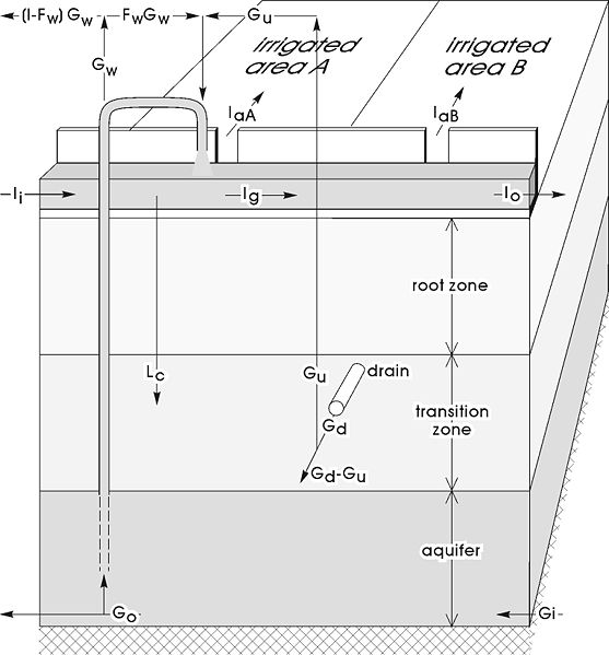
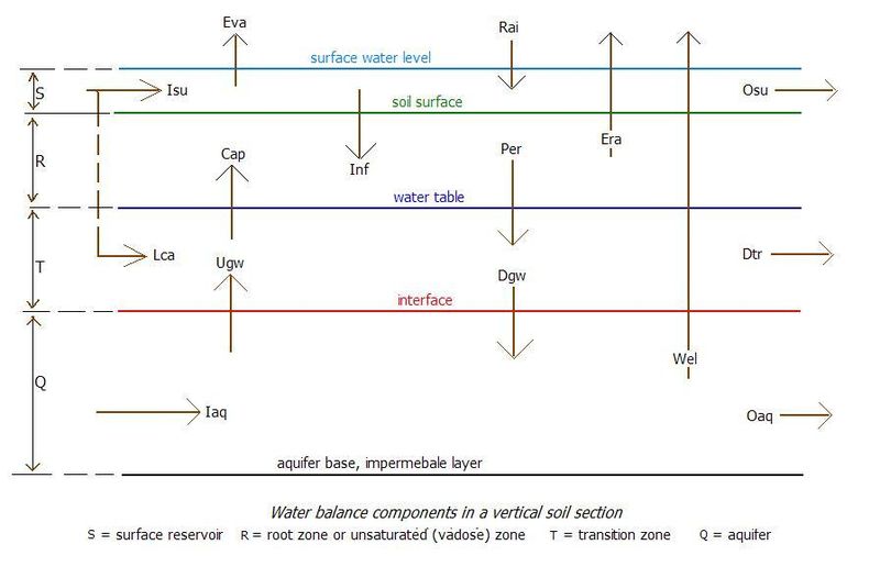
Sahysmod accepts four different reservoirs of which three are in the soil profile: - s: a surface reservoir - r: an upper (shallow) soil reservoir or root zone - t: an intermediate soil reservoir or transition zone - q: a deep reservoir or main aquifer. The upper soil reservoir is defined by the soil depth, from which water can evaporate or be taken up by plant roots. It can be taken equal to the root zone. It can be saturated, unsaturated, or partly saturated, depending on the water balance. All water movements in this zone are vertical, either upward or downward, depending on the water balance. (In a future version of Sahysmod, the upper soil reservoir may be divided into two equal parts to detect the trend in the vertical salinity distribution.) The transition zone can also be saturated, unsaturated or partly saturated. All flows in this zone are horizontal, except the flow to subsurface drains, which is radial. If a horizontal subsurface drainage system is present, this must be placed in the transition zone, which is then divided into two parts: an upper transition zone (above drain level) and a lower transition zone (below drain level). If one wishes to distinguish an upper and lower part of the transition zone in the absence of a subsurface drainage system, one may specify in the input data a drainage system with zero intensity. The aquifer has mainly horizontal flow. Pumped wells, if present, receive their water from the aquifer only. The flow in the aquifer is determined in dependence of spatially varying depths of the aquifer, levels of the water table, and hydraulic conductivity. SAHYSMOD permits the introduction of phreatic (unconfined) and semi-confined aquifers. The latter may develop a hydraulic over or under pressure below the slowly permeable top-layer (aquitard). 2.8. Agricultural water balances The agricultural water balances are calculated for each soil reservoir separately. The excess water leaving one reservoir is converted into incoming water for the next reservoir. The three soil reservoirs can be assigned different thickness and storage coefficients, to be given as input data. When, in a particular situation the transition zone or the aquifer is not present, they must be given a minimum thickness of 0.1 m. |
|
Under certain conditions, the height of the water table influences the water-balance components. For example a rise of the water table towards the soil surface may lead to an increase of capillary rise, actual evaporation, and subsurface drainage, or a decrease of percolation losses. This, in turn, leads to a change of the water-balance, which again influences the height of the water table, etc. This chain of reactions is one of the reasons why Sahysmod has been developed into a computer program, in which the computations are made day by day to account for the chain of reactions with a sufficient degree of accuracy.
2.9. Ground water flow
The model calculates the groundwater levels and the incoming and outgoing ground water flows between the polygons by a numerical solution of the well-known Boussinesq equation. The levels and flows influence each other mutually.
The groundwater situation is further determined by the vertical recharge that is calculated from the agronomic water balances. These depend again on the levels of the ground water.
When semi-confined aquifers are present, the resistance to vertical flow in the slowly permeable top-layer and the overpressure in the aquifer, if any, are taken into account.
Hydraulic boundary conditions are given as hydraulic heads in the external nodes in combination with the hydraulic conductivity between internal and external nodes. If one wishes to impose a zero flow condition at the external nodes, the conductivity can be set at zero.
Further, aquifer flow conditions can be given for the internal nodes. These are required when a geological fault line is present at the bottom of the aquifer or when flow occurs between the main aquifer and a deeper aquifer separated by a semi-confining layer.
2.10 Drains, wells, and re-use
The sub-surface drainage can be accomplished through drains or pumped wells.
The subsurface drains, if any, are characterised by drain depth and drainage capacity. The drains are located in the transition zone. The subsurface drainage facility can be applied to natural or artificial drainage systems. The functioning of an artificial drainage system can be regulated through a drainage control factor.
By installing a drainage system with zero capacity one obtains the opportunity to have separate water and salt balances in the transition above and below drain level.
The pumped wells, if any, are located in the aquifer. Their functioning is characterised by the well discharge.
The drain and well water can be used for irrigation through a (re)use factor. This may have an impact on the water and salt balance and on the irrigation efficiency or sufficiency.
|
2.11 Salt balances The salt balances are calculated for each soil reservoir separately. They are based on their water balances, using the salt concentrations of the incoming and outgoing water. Some concentrations must be given as input data, like the initial salt concentrations of the water in the different soil reservoirs, of the irrigation water and of the incoming groundwater in the aquifer. The concentrations are expressed in terms of electric conductivity (EC in dS/m). When the concentrations are known in terms of g salt/l water, the rule of thumb: 1 g/l -> 1.7 dS/m can be used. Usually, salt concentrations of the soil are expressed in ECe, the electric conductivity of an extract of a saturated soil paste. In Sahysmod, the salt concentration is expressed as the EC of the soil moisture when saturated under field conditions. As a rule, one can use the conversion rate EC : ECe = 2 : 1. Salt concentrations of outgoing water (either from one reservoir into the other or by subsurface drainage) are computed on the basis of salt balances, using different leaching or salt mixing efficiencies to be given with the input data. The effects of different leaching efficiencies can be simulated varying their input value. If drain or well water is used for irrigation, the method computes the salt concentration of the mixed irrigation water in the course of the time and the subsequent impact on the soil and ground water salinity, which again influences the salt concentration of the drain and well water. By varying the fraction of used drain or well water (through the input), the long term impact of different fractions can be simulated. The dissolution of solid soil minerals or the chemical precipitation of poorly soluble salts is not included in the computation method. However, but to some extent, it can be accounted for through the input data, e.g. increasing or decreasing the salt concentration of the irrigation water or of the incoming water in the aquifer. In a future version, the precipitation of gypsum may be introduced. |
|
2.12 Farmers' responses
If required, farmers' responses to water logging and salinity can be automatically accounted for. The method can gradually decrease:
-1. the amount of irrigation water applied when the water table becomes shallower depending
on the kind of crop (paddy rice and non-rice)
-2. the fraction of irrigated land when the available irrigation water is scarce;
-3. the fraction of irrigated land when the soil salinity increases; for this purpose, the salinity is given a stochastic interpretation;
-4. the ground-water abstraction by pumping from wells when the water table drops.The farmers' responses influence the water and salt balances, which, in turn, slows down
the process of water logging and salinization. Ultimately a new equilibrium situation will arise.
The user can also introduce farmers' responses by manually changing the relevant input data. Perhaps it will be useful first to study the automatic farmers' responses and their effect first and thereafter decide what the farmers' responses will be in the view of the user.
2.13 Annual input changes
The program runs either with fixed input data for the number of years determined by the user. This option can be used to predict future developments based on long-term average input values, e.g. rainfall, as it will be difficult to assess the future values of the input data year by year.
The program also offers the possibility to follow historic records with annually changing input values (e.g. rainfall, irrigation, cropping rotations), the calculations must be made year by year. If this possibility is chosen, the program creates a transfer file by which the final conditions of the previous year (e.g. water table and salinity) are automatically used as the initial conditions for the subsequent period. This facility makes it also possible to use various generated rainfall sequences drawn randomly from a known rainfall probability distribution and to obtain a stochastic prediction of the resulting output parameters.
Some input parameters should not be changed, like the nodal network relations, the system geometry, the thickness of the soil layers, and the total porosity, otherwise illogical jumps occur in the water and salt balances. These parameters are also stored in the transfer file, so that any impermissible change is overruled by the transfer data. In some cases of incorrect changes, the program will stop and request the user to adjust the input.
2.14 Output data
The output is given for each season of any year during any number of years, as specified with the input data. The output data comprise hydrological and salinity aspects. The data are filed in the form of tables that can be inspected directly, through the user menu, that calls selected groups of data either for a certain polygon over time, or for a certain season over the polygons. Also, the program has the facility to store the selected data in a spreadsheet format for further analysis and for import into a mapping program. A user interface to assist with the production of maps of output parameters is still in development.
The program offers only a limited number of standard graphics, as it is not possible to foresee all different uses that may be made. This is the reason why the possibility for further analysis through spreadsheet program was created. The interpretation of the output is left entirely to the judgement of the user.
|
2.15 Other users' suggestions The program offers the possibility to develop a multitude of relations between varied input data, resulting outputs and time. Different users may wish to establish different cause and effect or correlation relationships. If the user wishes to determine the effect of variations of a certain parameter on the value of other parameters, the program must be run repeatedly according to a user-designed scenario. This procedure can be used for the calibration of the model or for the simulation runs. Some of the input data are inter-dependent. These data can, therefore, not be indiscriminately varied. In very obvious illogical combinations of data, the program will give a warning. The correctness of the input remains the responsibility of the user. Although the computations are done on a daily basis, all the seasonal end-results can be checked by hand with the equations given in the following sections because all output results are based on weighed seasonal averages. The size of the total area and the individual polygons can be determined at will by the user. When the topography and other conditions are fairly uniform, the total size of the area can be taken quite large, say 100 000 ha or more. For sloping or undulating lands, it deserves recommendation to use smaller areas. If necessary, the total area can be divided into sub-areas to which Sahysmod can be applied separately. It is of course also possible to use Sahysmod in smaller areas of 100 ha or less. In such areas fine-tuning of the model is feasible. The exercise and case study (given in sect. 12 and 13) refer to relatively small areas. Otherwise the examples would become too elaborate. |
|