SegRegA :   segmented regression with breakpoint as well as generalized S-curve and polynomial functions.
Totally free download of software

Summary: The SegRegA computer program (calculator) is designed to perform a segmented regression analysis, but in addition it offers the opportunity to apply S-curve, Power function, and polynomial regressions. These acquire an increased versatility through generalization by applying an exponential transformation of the data by assuming a range of exponents and selecting the one that produces the best fit. Thus, the exponent is optimized. The model recognises polynomials with 3 and 4 terms. The 3-term polynomial has the equation: Y = B.X^Q + C.X^R + D. It is found by transforming the X value raising it to the power E, which is to be optimized, obtaining the variable W = X^E and performing a quadratic (2nd degree) regression of Y upon W. This will result n the equation: Y = B.W^2 + C.W + D. Substituting herein W = X^E, Q=2E and R=E will provide the earlier mentioned equation in X, in which the powers Q and R can be different from 2 and 1 respectively. The 4-term polynomial has the equation: Y = A.X^P + B.X^Q + C.X^R + D. It is found likewise by transforming the X value raising it to the power E, which is to be optimized, obtaining the variable W = X^E and performing a cubic (3rd degree) regression of Y upon W. This will result in the equation: Y = A.W^3 + B.W^2 + C.W + D. Substituting herein the values W = X^E, P=3E, Q=2E and R=W will provide the earlier mentioned equation in X, in which the powers P, Q and R can be different from 3, 2 and 1 respectively. The optimal value of the exponent E is found by assuming a range of E values and selecting the one producing the best fit, i. e. the least sum of squares of deviations of calculated Y from observed Y values. The calculation of the cubic regression is complicated as it needs matrices and determinants leading to a large number of calculations. After all, the resulting polynomial equations are no longer quadratic or cubic. See the examples below. It may be noted that polynomial regression can also be of the linear type: Y = A.X + B.Z + C (polynomial). Examples of SegReg for such types are shown at the end of this page. Experiences: For improvement, I am interested to learn about your experiences with SegRegA. For this there is a contact form.                         Screenprint of SegRegA showing the regression options.

Download: SegRegA Go to: Software & models General articles & manuals Artiículos (in Spanish, en Español) Published reports & cases Particular reports & cases FAQ's & answers Home page

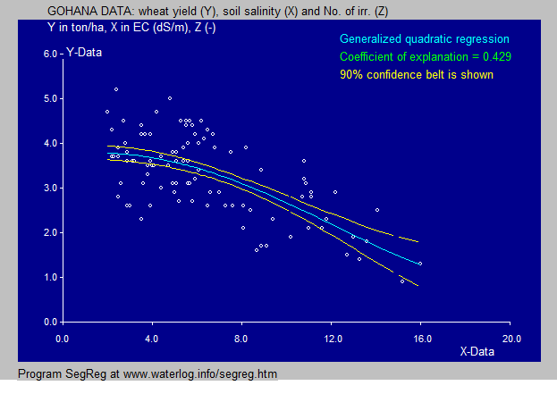
The quadratic equation in the wheat example is found by a transformation raising X to the power 2 so that W = X ^ 2 and then performing a quadratic regression of Y on W with the result: Y = 0.000126 W ^ 2 - 0.0120 W + 3.80 and hence: Y = 0.000126 X ^ 4 - 0.0120 X ^2 + 3.80 which is now no longer a second degree (quadratic) equation, but a 4th degree one.

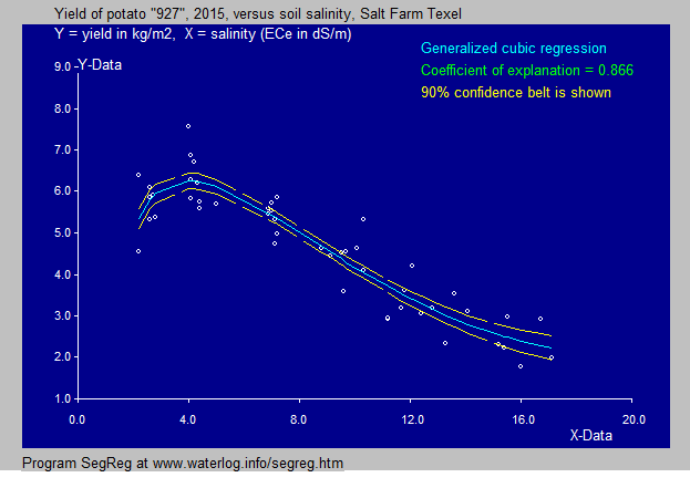
The cubic equation in the potato example is found by a transformation raising X to the power 0.5 so that W = X ^ 0.5 and then performing a cubic regression of Y on W with the result: Y = 0.537 W ^ 3 - 4.70 W ^ 2 + 11.2 W + 1.84 and hence: Y = 0.537 X ^ 1.5 - 4.70 X + 11.2 X ^ 0.5 + 1.84 which is now no longer a third degree (cubic) equation.

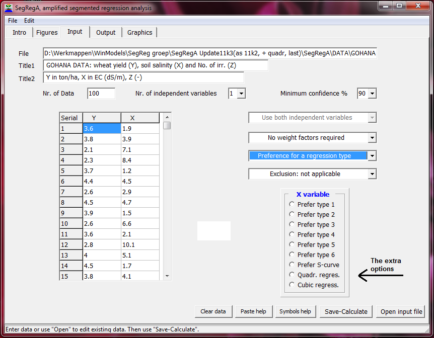
At a certain stage, the program asks if the transformation is OK (see figure below). If the answer is "No" then the standard quadratic or cubic regression will be made. Otherwise, the transformation may occur and it can be noted that the resulting equation is no longer a standard quadratic or cubic function, but that the exponents of the X-values have been changed to other values than the standard 3, 2 and 1. They have been generalized and the goodness of fit has increased.

The polynomal case of 1 dependent variable (Y) and 2 independent variables (X and Z)

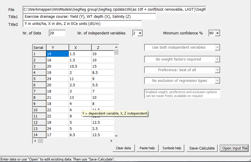
Screen print of the input menu for the polynomial case (1 dependent variable (Y) and 2 independent variables (X and Z).

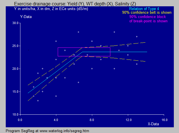
The SegReg program found that the 1st independent variable (X) has a higher coefficient of explanation than the second (Z). Therefore the first segemented regression is made for X.

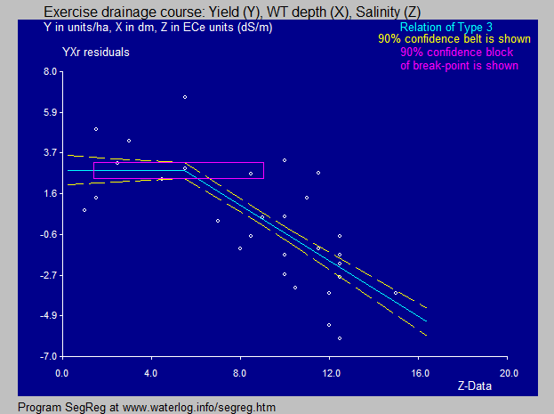
The the residuals of Y after the regression on X are used with a segmented regression on the second variable (Z). The mathematical combination of the first and second analysis yields equations of the type Y = A.X + B.Z + C (polynomial)